Infinitesimal Deformation Linear Elastic Static Analysis

In this section, the elastic static analysis is formulated on the basis of the infinitesimal deformation theory, which assumes linear elasticity as a stress-strain relationship.

Basic equations

The equilibrium equation, mechanical boundary conditions, and geometric boundary conditions (basic boundary conditions) of solid mechanics are given by the following equations (see Fig. 2.1.1):

\[\begin{equation} \nabla \cdot \sigma + \overline{b} = 0 \quad in \ V \label{eq:2.1.1} \end{equation}\]

\[\begin{equation} \sigma \cdot n = \overline{t} \quad on \ S_t \label{eq:2.1.2} \end{equation}\]

\[\begin{equation} u = \overline{u} \quad on \ S_u \label{eq:2.1.3} \end{equation}\]

where \(\sigma\), \(\overline{t}\) and \(S_t\) denote stress, surface force, and body force, respectively. \(S_t\) and \(S_u\) represent the geometric and mechanical boundaries, respectively.

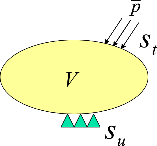
Fig. 2.1.1 Boundary value problem in solid mechanics (infinitesimal deformation problem)

The strain-displacement relation in infinitesimal deformation problems is given by the following equation:

\[\begin{equation} \varepsilon = \nabla_S u \label{eq:2.1.4} \end{equation}\]

Furthermore, the stress-strain relationship (constitutive equation) in linear elastic bodies is given by the following equation:

\[\begin{equation} \sigma = C : \varepsilon \label{eq:2.1.5} \end{equation}\]

where, \(C\) is a fourth-order elasticity tensor.

Principle of Virtual Work

The principle of the virtual work related to the infinitesimal deformation linear elasticity problem, which is equivalent to the basic equation Eq.\(\eqref{eq:2.1.1}\), Eq.\(\eqref{eq:2.1.2}\) and Eq.\(\eqref{eq:2.1.3}\), is expressed as:

\[\begin{equation} \int_V \sigma : \delta \varepsilon\, dV = \int_{S_t} \overline{t} \cdot \delta u\, dS + \int_V \overline{b} \cdot \delta u\,dV \label{eq:2.1.6} \end{equation}\]

\[\begin{equation} \delta u = 0 \quad on \ S_u \label{eq:2.1.7} \end{equation}\]

Moreover, considering the constitutive equation Eq.\(\eqref{eq:2.1.5}\), Eq.i\(\eqref{eq:2.1.6}\), is expressed as follows:

\[\begin{equation} \int_V (C : \varepsilon) : \delta \varepsilon\, dV = \int_{S_t} \overline{t} \cdot \delta u\, dS + \int_V \overline{b} \cdot \delta u\, dV \label{eq:2.1.8} \end{equation}\]

In Eq.\(\eqref{eq:2.1.8}\), \(\varepsilon\) is the strain tensor and \(C\) is the fourth-order elasticity tensor. In this case, if the strain tensor \(\sigma\) and \(\varepsilon\) are represented by vector formats \(\hat{\sigma}\) and \(\hat{\varepsilon}\), respectively, the constitutive equation Eq.\(\eqref{eq:2.1.5}\) is expressed as follows

\[\begin{equation} \hat{\sigma} = D \hat{\varepsilon} \label{eq:2.1.9} \end{equation}\]

where \(D\) is an elastic matrix.

Considering that the \(\hat{\sigma}\), \(\hat{\varepsilon}\) and Eq.\(\eqref{eq:2.1.9}\) are expressed in vector format, Eq.\(\eqref{eq:2.1.8}\) is expressed as follows:

\[\begin{equation} \int_V \hat{\varepsilon}^T D \delta \hat{\varepsilon}\, dV = \int_{S_t} \delta u^T \overline{t}\, dS + \int_V \delta u^T \overline{b}\, dV \label{eq:2.1.10} \end{equation}\]

Eq.\(\eqref{eq:2.1.10}\) and Eq.\(\eqref{eq:2.1.7}\) are the principles of the virtual work discretized in this development code.

Formulation

If the principle of virtual work, Eq.\(\eqref{eq:2.1.10}\), is discretized for each finite element, the following equation is obtained:

\[\begin{equation} \sum_{e} = \int_{V^e} \hat{\varepsilon}^T D \delta \hat{\varepsilon}\, dV = \sum_{e} \int_{S^e_t} \delta u^T \overline{t}\, dS + \sum_{e} \int_{V^e} \delta u^T \overline{b}\,dV \label{eq:2.1.11} \end{equation}\]

Using the displacement of the nodes that compose each element, the displacement field is interpolated as follows:

\[\begin{equation} u = \sum^m_{i=1} N_i u_i = N U \label{eq:2.1.12} \end{equation}\]

The strain at this moment, using Eq.\(\eqref{eq:2.1.4}\), is given as follows:

\[\begin{equation} \hat{\varepsilon} = B U \label{eq:2.1.13} \end{equation}\]

When Eq.\(\eqref{eq:2.1.12}\) and Eq.\(\eqref{eq:2.1.13}\) are substituted into Eq.\(\eqref{eq:2.1.11}\), the following equation is obtained:

\[\begin{equation} \sum_e \delta U^T \left( \int_{V^e} B^T DB\, dV \right) U = \sum_e \delta U^T \cdot \int_{S_t^e} N^T \overline{t}\, dS + \sum_{e} \delta U^T \int_{V^e} N^T \overline{b}\, dV \label{eq:2.1.14} \end{equation}\]

Eq.\(\eqref{eq:2.1.14}\) can be summarized as

\[\begin{equation} \delta U^T K U = \delta U^T F \label{eq:2.1.15} \end{equation}\]

In this case, the components of the matrix and vector defined by Eq.\(\eqref{eq:2.1.16}\) and Eq.\(\eqref{eq:2.1.17}\) can be calculated for each finite and overlapped element:

\[\begin{equation} K = \sum_e \int_{V^e} B^T DB dV \label{eq:2.1.16} \end{equation}\]

\[\begin{equation} F = \sum_e (\int_{S_t^e} N^T \overline{t}\, dS + \int_{V^e} N^T \overline{b}\, dV ) \label{eq:2.1.17} \end{equation}\]

if Eq.\(\eqref{eq:2.1.15}\) is true for an arbitrary virtual displacement \(\delta U\), the following equation is obtained:

\[\begin{equation} K U = F \label{eq:2.1.18} \end{equation}\]

Meanwhile, the displacement boundary condition Eq.\(\eqref{eq:2.1.3}\) is expressed as follows:

\[\begin{equation} U = \overline{U} \label{eq:2.1.19} \end{equation}\]

By solving Eq.\(\eqref{eq:2.1.18}\) based on the constraint condition Eq.\(\eqref{eq:2.1.19}\), it is possible to define the node displacement \(U\).